

Reference Publication: Parker, D., Dunlop, J., "Solar Photovoltaic Air Conditioning of Residential Buildings", Technology Research, Development and Evaluation 3 Proceedings, ACEEE 1994, Summer Study on Energy Efficiency in Buildings, August 1994. Disclaimer: The views and opinions expressed in this article are solely those of the authors and are not intended to represent the views and opinions of the Florida Solar Energy Center. |
Solar Photovoltaic Air Conditioning of Residential Buildings
Danny
S. Parker and James P. Dunlop
Florida
Solar Energy Center (FSEC)
FSEC-RR-118-94
The use of photovoltaics
(PV) for residential air conditioning (AC) represents an attractive application
due to the close match between the diurnal cooling load and the availability
of solar radiation. Conventional wisdom suggests that air conditioning
is a process too energy intensive to be addressed by PV. Previous investigations
have concentrated on the feasibility of matching PV output to vapor-compression
machines, and the cost effectiveness of other solar cooling options. Recently,
Japanese manufacturers have introduced small (8,000 Btu/hr) grid-connected
solar assisted AC systems. These small room-sized systems are inadequately
sized to meet air conditioning peak demands in larger U.S. homes of conventional
construction practice. Previous studies considering the use of PV for solar
cooling have treated the building thermal load as a fixed quantity. However,
the large initial cost of PV systems ($6 - $lO/Wpeak) makes minimization
of the building loads highly desirable. This paper describes a novel approach
whereby the building, air conditioning and PV systems are simultaneously
optimized to provide maximum solar cooling fraction for a minimum array
size.
A detailed hourly building energy simulation in a hot-humid climate
is used to assess methods of reducing the building sensible and latent cooling
loads to a practical minimum. A detailed PV system simulation is used to
determine the match of the array output to that of the building’s peak
loads. The paper addresses several key elements that influence the concept’s
feasibility and potential economic attractiveness.
Introduction
The few prior
studies of PV-powered AC have concentrated on the feasibility of matching
PV output to vapor- compression machines, and the cost-effectiveness of
competing options [Kern 1979; Stephens et al., 1980]. Recently, three Japanese
manufacturers have announced commercialization and test results for small
(8500 Btu/hr) grid-connected PV assisted AC systems Tanaka et al., 1990;
Sawai 1992; Takeoka et al., 1993]. In the United States, the Electric Power
Research Institute is testing PVpowered heat pumps [EPRI 1993].
All previous investigations considering the use of PV for solar cooling
of buildings have treated the building thermal load as a fixed quantity.
However, the large initial cost of PV systems ($61O/Wpeak) makes minimizing
the building load highly desirable. A number of conservation measures can
decrease the load at a lower cost than the load can be satisfied with PV.
Substantial reductions are therefore possible in the required PV system and
AC unit size, and the thermal delivery system. One limitation, however, is
that the approach would be practical only for new home construction. Initially,
three fundamental cases were defined to characterize residential electrical
load profiles:
- Base
Residential Building: This case represents current building
construction practice and employs standard efficiency electrical
appliances and HVAC equipment.
- Minimum
Cooling Energy Residential Building: This case represents an all-electric
residence with thermally optimized construction and incorporates all
available methods to reduce building cooling and electrical loads.
- Minimum Electricity Residential Building: This case is identical to case 2 except that natural gas is used instead of electricity for appropriate end-use appliances.
Base
Residential Building
A prototype building, typical of residences in southern climates,
was used to define characteristics for the base residential building
[Fairey et al., 19861. Table 1 summarizes the assumptions.
Three occupants were assumed in the prototype residence with typical
electrical appliances. The specific end-use electrical demand profiles were
taken from sub-metered appliance load data gathered from a large sample of
homes during the summer months [Pratt et al., 1989]. The hot water electrical
demand profile was based on measured data collected on 18 electric resistance
water heaters in Florida [Merrigan 1983].
Table 1. Building System Specifications Base Residential Building
|
||||||||||||||||||||||||||||||||||||||||||||||||||||||||||||
Minimum
Cooling Energy Residential Building
Energy efficient improvements to the building envelope result
in significant AC load reductions. These improvements include wall
and ceiling insulation, white exterior walls, a reflective roof, reflective
windows, landscape shading of walls and windows, and a ductless AC
system [Fairey et al., 1986; Parker 1990; Parker et al., 1992; Parker
et al., 1993]. Internal heat gains represent the largest component
of the AC load in typical, well- insulated residential buildings. Accordingly,
the minimum cooling energy building features a variety of proven technologies
to reduce the internal load from appliances and lighting. Table 2 summarizes
the methods (and their cost) used to reduce the base residential building
AC load to the minimum cooling energy building AC load.
The AC load conservation measures presented above behave according
to a law of diminishing returns: decreased savings are realized from each
additional measure implemented. Figure 1 shows how the minimum cooling energy
building was optimized by adding the most effective options in order of their
incremental contribution to reducing the peak day cooling load (optimization
by steepest descent).
Minimum Electricity Residential Building
Methods were also examined to reduce the overall building electrical
loads to a practical minimum. This was accomplished by substituting non-electric
fuels in place of electrical appliances where applicable. For the minimum
electric residential profile described here, solar for water heating with
natural gas backup and natural gas for cooking, heating and clothes drying
are used instead of electricity. In an all-electric residence, these appliances
result in peak load demands over short periods. By substituting gas or alternative
fuels, the peak load can be satisfied by a smaller PV system than would be
required for the all-electric residence.
Table 2. Thermal Efficiency Improvements: Methods and Cost Minimum Cooling Energy Building
|
|||||||||||||||||||||||||||||||||||||||||||||||||||||||||||||||||||||||||||||||||||||||
Building
System Analysis
For the three residential cases presented above, an hourly
building energy simulation program, FSEC 2.1, was used to
compute hourly electrical demand profiles for both the AC and appliance
loads [Kerestecioglu et al., 1989].
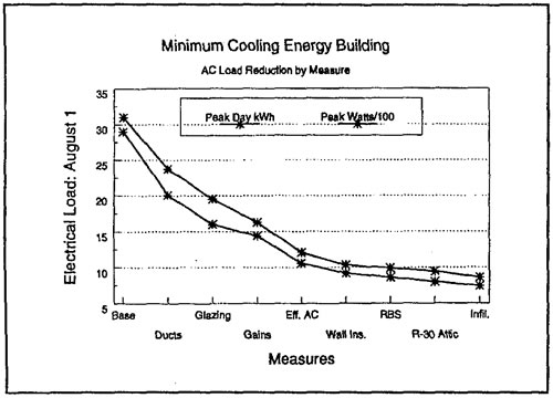
Figure 1. Energy Conservation Measures for Minimum
Cooling Energy Building
The building
load simulation, as well as the subsequent PV system modelling were performed
using Typical Meteorological Year (TMY) data for Orlando, Florida [TMY
User’s Manual 1981]. The cooling-dominated Central Florida climate
was used since it induces in an extreme AC load. In addition, the variability
of summer afternoon insolation suggests examining the match between peak
residential AC loads and PV system performance.
Figure 2 summarizes key climatic data for the year; Figure 3 presents
the hourly average temperature, insolation, relative humidity and wind speed
for the summer peak cooling load day of August 1st.
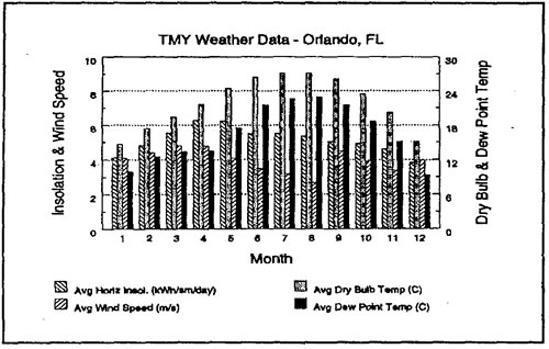
Figure 2. Annual Weather Data for Orlando, FL.
Table 3 summarizes the annual results of the FSEC 2.1 simulations for the three residential building load cases. Predictions for the base case (11,312 kWh/yr) were consistent with the mean energy consumption of 177 all- electric homes in Florida (12,900 kWh/yr) as measured in the field [Vieira and Parker 19911. The predicted AC loads were reduced from 2,968 kWh for the base case to only 681 kWh for the minimum cooling energy building. High-efficiency lighting, refrigeration and hot water conservation measures resulted in a reduction of appliance electricity use of 2,991 kWh for a total annual electrical savings of 5,277 kWh. At an energy cost of $0.07/kWh, these measures offer an annual savings of $369 with a simple payback of about 14 years.
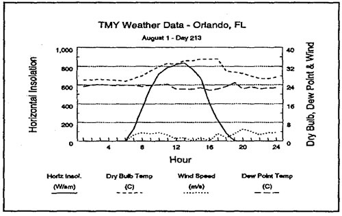
Figure 3. Weather Data for August 1st, Orlando,
FL.
Most notably,
the annual energy use for the minimum electricity residence was only 2,091
kWh-a decrease of 82% compared to the base case. These measures are able
to offset an estimated 3,859 kWh per year electrical demand (550 to 900
W peak) at an incremental cost of only $150. The electric savings are achieved
with the additional use of approximately 190 therms/yr of natural gas.
On the peak load day of August 1st, the AC energy consumption was reduced
from 31 kWh for the base case to below 8 kWh for the minimum cooling energy
building. The coincident peak AC load on the same day was reduced by over
2 kW.
The base case building had a maximum cooling load on August 1st of
8,292 W (28,300 Btu per hour) as compared to 2,461 W (8,400 Btulhour) for
the minimum cooling energy building. Clearly, the newly available small Japanese
AC units would be unable to adequately cool the base case house but could
theoretically provide the necessary cooling for the minimum cooling energy
building.
PV System Analysis
Several strategies are conceivable for integrating PV in residential
buildings to satisfy all or part of the loads. In a stand-alone configuration,
the PV system would be designed independent of the utility grid to interface
directly with the load or with battery storage. The loads would be operated
with de power, or with ac power with the use of a stand-alone inverter connected
to the battery. In a grid-connected or utility-interactive configuration,
a power conditioner is used to interface the PV array output with the utility.
The building load and PV array output then dictate the direction of energy
flow between the PV, load and utility.
Table 3. Summary of Building Electrical Loads
|
||||||||||||||||||||||||||||||
Both
the stand-alone and grid-connected configurations have been successfully
employed for residential power. Often, the PV array for grid-connected
residential systems is deliberately undersized to provide only peak load
reduction and is not sized to meet the entire load. The reasoning for undersizing
the PV array is due to the low value for energy sold to the utility as
compared to the high cost of PV generated energy.
For the analyses presented here, only grid-connected systems are considered.
Although not presented here, PV AC systems without the ability to either
serve other non- cooling loads or to sell-back electricity to the utility
appear impractical.
PV system characteristics typical of residential installations were
used for the analysis. It was assumed that the array was located on a south-facing,
200 roof slope. Furthermore, efficiencies typical of current PV systems technology
were used, including an array efficiency of 10% and a power conditioner (inverter)
efficiency of 90%.
The ability of PV systems to contribute capacity during the peak electrical
demand periods is of significant interest to electric utilities [Russell
and Kern 1992]. Our analysis seeks to define PV array sizes, electrical storage
requirements and utility rate structures that offer the best near- term market
for residential PV systems.
Preliminary Sizing Estimates
To attain a first approximation of the PV system sizes required to
meet the daily energy and 5-6 p.m. peak loads on the maximum cooling
load day of August 1st, the following equation was used:
A = L/ I na ns t
where
A = array size (m2)
L = design load (Wh)
I = avg insolation for period (W/m2)
a = array efficiency
s = storage/power conditioner efficiency
t = period of the insolation cycle (hrs)
For the daily
load, the insolation value of 6.35 kWh/m2 for August 1st on a south facing,
20° tilted surface was used to calculate the array size. For the 5-6
p.m. peak summer load period defined by Florida utilities, a value of 208
W/m2 was used to determine the required array size to meet the peak.
The daily and peak loads for August 1st, along with the required PV
array area to meet the daily energy and peak load are summarized in Table
4.
Table 4. Electrical Loads and Predicted Array Sizes, August 1 - Day 213
|
|||||||||||||||||||||||||||||||||
The results
show that a very large reduction in array size is possible through the
use of building improvements to reduce cooling loads. A considerably larger
PV array is needed to offset the 5-6 p.m. utility peak without
storage or utility backup. The array sizes required to meet the entire
base building loads are clearly impractical since the required collection
area may exceed that of an entire residential roof.
PV System Hourly Simulation
An obvious limitation of the above analysis is that it does not examine
how well the PV system output matches the coincident building load over the
entire year. To analyze the performance of different PV array sizes with
the three residential load profiles, the computer program PVFORM was
used to determine the hourly contributions of the PV array and utility (backup)
in meeting the load [Menicucci and Fernandez 1988]. Table 5 summarizes key
input parameters were used in the PVFORM simulations.
Table 5. PVFORM Input Parameters
|
Utility
Rate Calculations
Software was written to read the PVFORM hourly output
files and to analyze the effects of different utility rates, energy
storage and PV array sizes on the value of the energy bought from and
sold to the utility. The cost of electricity sold to and bought from
the utility were developed based on discussions with major electric
utilities in Florida. While the rates are not specific to a particular
utility, the rates are typical of what would be available to a residential
PV system owner. Three utility rates were defined for our analysis:
1. Co-Generation
Rate (Co-Gen)
Energy Bought From Utility ($IkWh) $0.070
Energy Sold To Utility (S/kWh) $0.030
2. Time-of-Use Rate (TOU)
Winter Peak Time: Nov.-Mar. 6am-l0am & 6pm-l0pm.
Summer Peak Time: Apr. -Oct. l2pm-9pm.
All other times off-peak.
Energy Bought
From Utility (On Peak, $/kWh) $0.079
Energy Bought From Utility (Off Peak, $/kWh) $0.027
Energy Sold To Utility (On Peak, $/kWh) $0.040
Energy Sold To Utility (Off Peak, s/kWh) $0.030
Analysis Results
Annual results for selected cases are presented as a series of tables. Table 6 examines the performance of a 1 kWp PV array as affected by the specific building use analyzed.
Table 6. Sensitivity of Annual Performance to Building Type (1 kWp PV, Co-Gen Rate)
|
|||||||||||||||||||||||||||||||||||||||||||||||||||||||||||||||||||||||
Table 7 illustrates the influence of array size on annual performance for the base building (AC load only).
Table
7. Sensitivity of Annual Performance to PV Array Size
(Base Building: AC only, Co-Gen Rate)
|
|||||||||||||||||||||||||||||||||||||||||||||||||||||||||||||||||||||||
Table 8 compares the performance of a 1 kW PV system with the Co-Gen rate and time-of-use rate (TOU) for both the AC and all electrical loads.
Table 8. Effect of Time-of-Use Rate on Annual Performance (1 kWp PV)
|
|||||||||||||||||||||||||||||||||||||||||||||||||||||||||||||||||||||||||||||||||||||||||||||||
Examination of these results leads to several conclusions:
- Building
efficiency has a profound effect on the ability of a PV array to
serve the AC load.
- Improvements
to building efficiency are currently more cost-effective than increasing
PV array size for reducing electrical loads.
- Time-of-use (TOU) electrical rates appear to be advantageous for PV grid-connected applications.
Figure 4 shows the August 1st AC load and the PV system performancc (0.5 and 2 kW arrays) for the base and minimum cooling energy buildings.
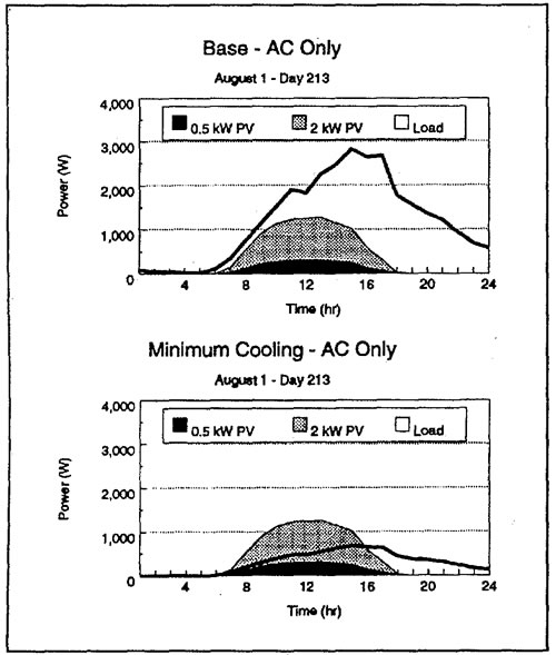
Figure 4. Air Conditioning Load and PV Output
for Base
and Minimum Cooling Energy Building, August 1st
Figure 5 presents the PV system performance (1 and 2 kW arrays) for all loads for the base and minimum electrical building cases.
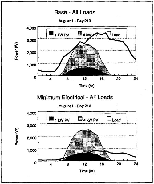
Figure 5. All Electrical Loads and PV Output for
Bas
and Minimum Electrical Energy Building, August 1st
Key findings from the examination of the load shape profiles (Figures 4 and 5) for the peak cooling load day of August 1St include:
- The
AC and overall building peak cooling load occurs approximately 4 hours
after the peak PV system output.
- The AC load
for the base building requires an array size of approximately 4 kW to
meet the majority of the peak load.
- The majority
of the AC load for the minimum cooling energy building can be met with
a 1 kW PV array. Also, the cooling load appears to closely match the
output of the PV system on the peak day.
- The electrical load of the minimum electricity residential building is best matched by a 1 kW array.
Conclusions
A fundamental objective of this study was to examine considerations
for using PV to satisfy residential AC loads. Perhaps the most significant
conclusion was that the required PV system size can be greatly reduced
by minimizing the building cooling load. Improvements to the building
envelope and appliances were able to decrease the cooling load by over
75%, reducing the required PV array size by a factor of four. At a
cost of approximately $5,100 for the improvements, this achieves a
load reduction more cost-effectively than by sizing the PV array to
meet the base case load. Given the seasonal nature of the cooling load,
it is apparent that a residential PV system be able to displace other
electrical loads during the non-summer months. A PV system that served
all building loads saved nearly twice as much in annual utility costs
than a system which powered the AC system only. In most cases, TOU
utility rates will be beneficial when used with residential PV systems.
In our analysis,
both the building and PV system simulations were driven by hourly weather
data. However, actual building electrical loads exhibit short-term “needle
peaks which can exceed the hourly average load profile. This problem is
greatest for buildings with all-electric appliances; therefore the analysis
presented here for the base case building must be considered somewhat optimistic.
Future analysis of PV AC systems should also consider how array axis-tracking,
load shifting, thermal or electrical storage and intelligent building systems
influence the ability of a PV system to meet the coincident peak loads. One
potentially attractive option would be to use the PV AC system to pre-cool
an exterior insulated masonry building in the non-peak morning hours. Another
option to the matching of PV array output with AC loads is to use a non-south
azimuth to delay the timing of maximum array output. For instance, based
on a combination of empirical data and simulation, Nawata (1992) showed that
the optimal orientation of a solar cooling system in Japan consisted of an
optimal azimuth approximately 20 degrees west of due south with an array
slope of latitude minus ten degrees. However, regardless of approach, a comprehensive
optimization of solar cooling systems suggests the use of analytical methods
which account for potential tradeoffs between building thermal efficiency,
array area, thermal storage capacity and other relevant parameters [Fukushima
et al., 1992].
A key question, not addressed by this preliminary study, is the cost-effectiveness
and practicality of the options considered. This may be appropriate after
further study has identified the most desirable system configurations (building
efficiency, PV size, thermal or electrical energy storage and operational
strategies). The life-cycle costs of the various options and hardware compatibilities
should then be examined. Finally, a full-scale demonstration of potentially
competitive configurations should be undertaken in residential buildings
to verify predicted results.
References
Electric Power Research Institute, 1993, “Central and
Southwest, Salt River Project Testing Solar Heat Pumps,” EPRI
News Exchange, Vol. 5, No. 3, Palo Alto, CA.
Fairey, P., Kerestecioglu, A., Vieira, R., Swami, M. and Chandra, S.,
1986. Latent and Sensible Distributions in Conventional and Energy Efficient
Residences, Gas Research Institute, FSEC-CR-153-86, Cape Canaveral,
FL.
Fukushirna, T., Sato, E. and Arai, N., 1993, “Optimum Design of Solar Powered Air Conditioning Systems,” Solar Engineering, Vol. 1, American Society of Mechanical Engineers, p. 229-234.
Grocoff, P.
N., 1990, “The Building Envelope and Photovoltaic Power as Tools
for Peak Shaving in Hot Arid Climates,” Proceedings of the 1990
Annual Conference of the American Solar Energy Society, ASES, Boulder,
CO.
Kern, E. C., “On Air Conditioning with Photovoltaics, 1979,” ASME
International Gas and Solar Conference, American Society of Testing
and Materials, San Diego, CA.
Kerestecioglu, A. Swami, M., Fairey, P., Gu, L. and Chandra, 5., 1989, “Modeling
Heat, Moisture and Contaminant Transport in Buildings: Towards a New Generation
Software,” ASHRAE Transactions, Vol. 95, Pt.2, Atlanta,
GA.
Menicucci, D. F., and Fernandez, J. P., 1988, User’s Manual for
PVFORM: A Photovoltaic System Simulation Program for Stand-Alone and Grid-Interactive
Applications, Report # SAND85-0376 UC-276, Sandia National Laboratories,
Albuquerque, NM.
Merrigan, T., 1983, Residential Conservation Demonstration: Domestic
Hot Water, Final Report, FSEC-CR-81- 29(RD), Florida Solar Energy Center,
Cape Canaveral, FL.
Nawata, Y., 1992, “Optimum Design of System Parameters for Solar Cooling
and Heating Aided by a Photovoltaic Array,” Solar Engineering, Vol.
1, American Society of Mechanical Engineers, p. 261-266.
Parker, D., Fairey, P. and Gu, L., 1993, “Simulation of the Effects
of Duct Leakage and Heat Transfer on Residential Space Cooling Energy Use,” Energy
and Buildings, 20, Elsevier Sequoia, Netherlands, p. 97-113.
Parker, D., Fairey, P., Gueymard, C., McCluney, R., Mcllvaine, 3. and
Stedman, T., 1992, Rebuilding for Efficiency: Improving the Energy Use
of Reconstructed Residences in South Florida, FSEC-CR-562-92, Florida
Solar Energy Center, Cape Canaveral, FL.
Parker, D. S., 1989, “Analysis of Annual and Peak Load Savings of High-Performance
Windows for the Florida Climate,” Proceedings of the Thermal Performance
of the Exterior Envelopes of Buildings IV, ASHRAE/DOE/ BTECC/CIBSE,
Orlando, FL, 1989.
Pratt, R. G. et al., 1989, Description of Electric Energy Use in Single-Family
Residences in the Pacific Northwest: End Use Load and Consumer Assessment
(EL CAP) Pacific Northwest Laboratory, Richiand, WA, July.
Russell, M.
C. and Kern, E. C., 1992, “Utility Interactive Residential PV: Lessons
Learned,” Solar Today, MayJune, P. 23-25.
Sawai, H., Okamoto, M., Kodarna, H., Matsuki, K., Ohmori, S. and Tsuyuguchi,
Y., 1992. “Residential Air Conditioning System with Photovoltaic Power
Supply,’ Solar Engineering, Vol. 1, American Society of Mechanical
Engineers, p. 273-277.
Stephens, W. H., McNeils, B., Naylor, A. I., and Brunt, P., 1980, ‘Photovoltaic
Systems for Cooling Applications,” Third European Communities Photovoltaic
Solar Energy Conference, D. Reidel Publishing Co, London.
Takeoka. A., Fukuda, Y., Suzuki, M., Hasunuma, M., Sakoguchi, E., Tokizaki,
H., Kouzuma, S., Waki, M., Ohnishi, M., Nakano, S. and Kuwano, Y., 1993, “Solar
Powered Air Conditioner,” Progress in Photovoltaics: Research and
Applications, Vol. 1, p. 47-54.
Tanaka, K.,
Toyoda, T., Waki, M., Sakoguchi, E, Yamada, M., Takeoka, A, Kishi, Y.,
Sakai, T. and Kuwano, Y., 1990, “Residential Photovoltaic System
with Air Conditioner,” Sanyo Electric Co., Ltd., Technical Digest
of the International PVSEC-5, Kyoto, Japan. Typical Meteorological
Year User’s Manual, 1981, National Climatic Data Center, Asheville,
NC, May.
Vieira, R. K., and Parker, D. S., 1991, Energy Attached and Detached
Residential Developments, CR-381-91, Florida Solar Energy Center, Canaveral,
FL.
© 2007-2014 University of Central Florida. The Florida Solar Energy Center (FSEC)
is a research institute of the
University of Central Florida.
For more information about FSEC, please contact us or learn more about us.
Find us on Facebook!